Friedman test
The Friedman test is a non-parametric statistical test used to compare the mean ranks of three or more related groups. It is similar to the one-way repeated measures ANOVA, but is used when the assumptions of normality and equal variances are not met.
“Whoa, whoa, wait a second!” I hear you exclaim, “That’s what you said about the Kruksal-Wallis test too!”
TL;DR The Friedman test is used for related groups with ordinal data, while the Kruskal-Wallis test is used for independent groups with ordinal data.
You would be right but there are a couple of key differences between the Friedman test and the Kruskal-Wallis test.
- Assumptions: The Friedman test assumes that the data are measured on an ordinal scale and that the observations within each group are related (i.e., repeated measures or matched pairs). The Kruskal-Wallis test assumes that the data are independent and identically distributed, and only requires that the groups be measured on an ordinal scale.
- Post-hoc tests: If the Friedman test or Kruskal-Wallis test shows that there is a significant difference between the groups, post-hoc tests can be used to determine which groups differ significantly from each other. The most common post-hoc test for the Friedman test is the Wilcoxon signed-rank test, while the most common post-hoc test for the Kruskal-Wallis test is the Dunn’s test.
The null hypothesis of the Friedman test is that there is no difference in the mean ranks of the groups.
The alternative hypothesis is that at least one group has a different mean rank than the others.
Example of when and how to use a Friedman tests
Imagine you are a music producer who wants to compare the popularity of three different music genres: hip-hop, rock, and country. You have surveyed 10 music fans and asked them to rate their preference for each genre on a scale of 1 to 10. You want to know if there is a significant difference in the mean preference for each genre, so you decide to use the Friedman test.
Your data should look something like this:
| Hiphop | Country | EDM | |
|---|---|---|---|
| Person 1 | 6 | 3 | 8 |
| Person 2 | 7 | 4 | 7 |
| Person 3 | 8 | 5 | 9 |
| Person 4 | 4 | 6 | 5 |
| Person 5 | 5 | 2 | 6 |
| Person 6 | 6 | 4 | 7 |
| Person 7 | 7 | 5 | 8 |
| Person 8 | 8 | 3 | 6 |
| Person 9 | 4 | 5 | 8 |
| Person 10 | 5 | 7 | 8 |
As you analyze the data, you notice that hip-hop is the most popular genre among young people, while rock is more popular among older fans. You also notice that there are some fans who rate all three genres equally, while others have a strong preference for one over the others.
When you run the Friedman test, the p-value returned is < 0.05 indicating a significant difference in the mean preference for each genre, indicating that some genres may be more popular than others among music fans. HOWEVER, you do not know who is different until you apply a post hoc test.
Post hoc test
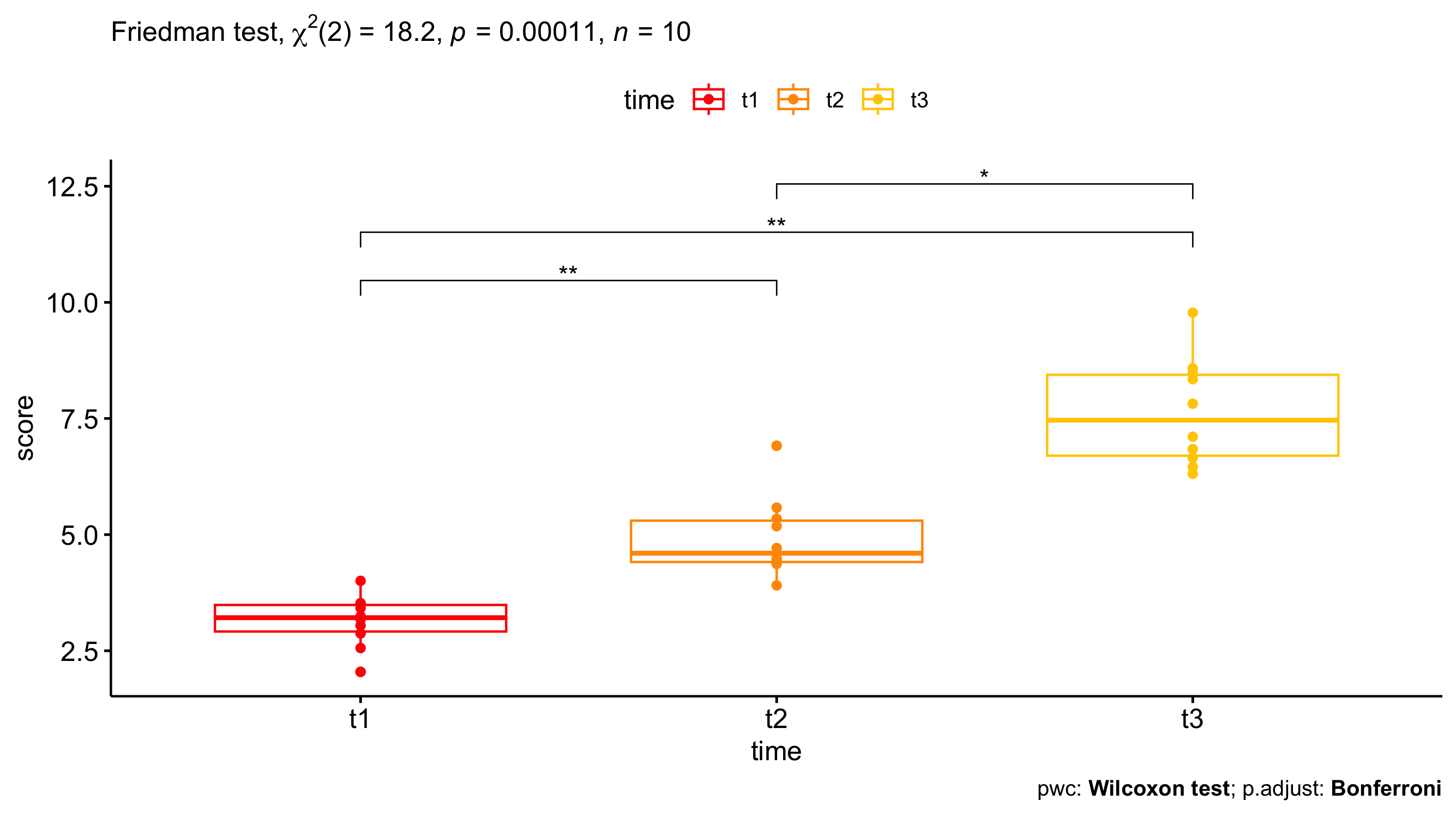
The most common post-hoc test for the Friedman test is the Wilcoxon signed-rank test. Briefly, the Wilcoxon signed-rank is a nonparametric test that can be effective at determining if paired data have different means. Much like the post hoc Tukey test following an ANOVA or a Dunn’s test following a Kruskal-Wallis test, you MUST perform the Wilcoxon signed-rank test to identify WHICH groups are different.
Visualizing the results
Just because you ran the analysis in JMP does not mean you have to use JMP to visualize your results. As long as you have a statistically significant result you can generate the plots however you would like (e.g., Excel, Google Sheets, R, Python). All you need to do is add an annotation to the figure that the P-value was < 0.05. A box-and-whisker plot would be a good way of visualizing the results of a Friedman test. The box-and-whisker plot would present both the spread of the data while also incorporating error bars associated with the mean calculation.
